
Design of a Technique for Analyzing Linear Time-Invariant Systems with Time-Varying Parameters Using Laplace Transform
Team: Junhan Chen, Shengda Gao, Yiwen Wang, Yulin Xia, Yang Tian, Siyuan Lin
Course: MTH101 Engineering Mathematics
Institution: Xi’an Jiaotong-Liverpool University
Date: Oct 2024 – Dec 2024
Background
Linear Time-Invariant (LTI) systems are fundamental in control systems, signal processing, and communications. Traditional analysis assumes constant system parameters, which often fails to reflect real-world variations. In practical systems, parameters may fluctuate due to external disturbances or internal dynamics. For example, the stiffness of a spring or the damping coefficient of a mechanical system may vary with time.
Various approaches such as time-varying control and adaptive control have been proposed to address parameter variations. However, these approaches may introduce significant complexity and computational cost.
During this course, the Laplace Transform was studied as a mathematical tool capable of converting differential equations from the time domain into algebraic equations in the frequency domain. In this project, the Laplace Transform is extended to handle time-varying parameters through the introduction of a Modified Laplace Transform (MLT), allowing LTI systems to capture time-variant behaviour more effectively.
Description of the Model
1. Introduction of the Formula in this Report
(1) Laplace Transform
The Laplace Transform is an integral transform widely used in engineering mathematics. It converts a function of time (t) into a function of a complex variable (s).
For a function (f(t)), the Laplace Transform is defined as
\[F(s) = \int_{0}^{\infty} f(t)e^{-st}dt\]This transformation converts differential equations into algebraic equations in the frequency domain, making it easier to analyse system behaviour.
(2) Modified Laplace Transform
In this report, the concept of a Modified Laplace Transform (MLT) is introduced to evaluate LTI systems with time-varying parameters.
To derive the modified formulation, the Laplace Transform is applied to both sides of the governing function. This leads to the expression
\[-\frac{d}{ds}\left(s^2Y(s)-sy(0)-y'(0)\right) +\frac{d}{ds}\left(sY(s)-y(0)\right) -2\left(sY(s)-y(0)\right)+2Y(s)=0\]which can be simplified to
\[\frac{dY(s)}{ds}+\frac{4s-3}{s(s-1)}Y(s)=\frac{3y(0)}{s(s-1)}\]An integrating factor is then introduced
\[\mu(s)=s^3(s-1)\]Multiplying both sides by the integrating factor gives
\[\frac{d}{ds}\left(Y(s)s^3(s-1)\right)=3s^2y(0)\]Integrating with respect to (s) results in
\[Y(s)=\frac{y(0)}{s-1}-K\left(\frac{1}{s}-\frac{1}{s^2}+\frac{1}{s^3}-\frac{1}{s-1}\right)\]Finally, the inverse transform is applied to obtain the solution in the time domain.
2. Why Building This Model and How to Use It
This study focuses on LTI systems whose parameters fluctuate over time. Traditional LTI analysis assumes constant parameters, which may not accurately represent real dynamic systems.
Using the Modified Laplace Transform (MLT), differential equations with time-varying coefficients can be analysed more effectively. The method captures dynamic parameter changes and allows the system behaviour to be studied under varying conditions.
The approach provides a framework for analysing systems with time-dependent transfer functions while maintaining the analytical advantages of transform methods.
3. Testing the Effectiveness of This Method in Solving Problems
To verify the effectiveness of the Modified Laplace Transform method, the inverse transform is applied to recover the time-domain solution (y(t)).
By applying the inverse MLT to each term of the expression for (Y(s)), the system response in the time domain can be obtained. This demonstrates that the method provides a systematic approach for analysing LTI systems with time-varying parameters.
The flexibility of the MLT makes it a useful analytical tool for studying dynamic systems with variable coefficients.
Explanation
1. A Spring-Mass Damper System
To illustrate the modelling framework, a spring-mass-damper system with time-varying parameters is analysed.
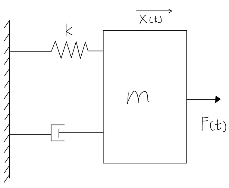
The governing differential equation of the system is
\[F(t)=m\frac{d^2X(t)}{dt^2}+b\frac{dX(t)}{dt}+kX(t)\]where
- (F(t)) is the applied force
- (X(t)) is the displacement
The system parameters are defined as
\[m=\cos(t)\] \[k=3\cos(t)\] \[b=-2\sin(t)\]The applied force is
\[F(t)=2u(t)\]Applying the Laplace Transform to both sides of the equation and simplifying (assuming zero initial conditions) allows the system behaviour to be analysed in the frequency domain.
Numerical Verification
MATLAB simulations are used to verify whether the proposed approach captures the dynamic behaviour of the system.
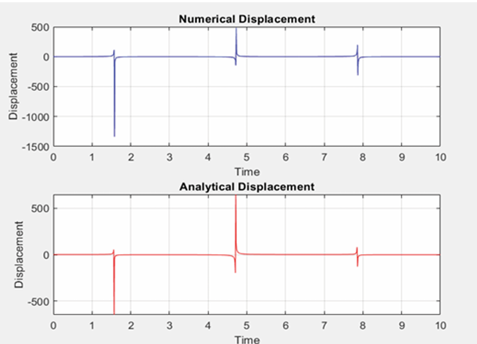
The first plot represents the numerical displacement, while the second plot represents the analytical displacement derived from the mathematical model.
Since the two curves show strong agreement, the results indicate that the method is capable of capturing the system dynamics accurately.
2. Handling LTI Systems with Time-varying Parameters
An LTI system with time-varying parameters can be represented by a differential equation with variable coefficients
\[y''(t)+a(t)y'(t)+b(t)y(t)=u(t)\]Using the Modified Laplace Transform, each term can be transformed into the frequency domain. Let
- (Y(k)) be the MLT of (y(t))
- (U(k)) be the MLT of (u(t))
Applying MLT properties gives
\[k^2Y(k)-ky(0)-y'(0)+a(k)[kY(k)-y(0)]+b(k)Y(k)=U(k)\]Solving the equation leads to
\[Y(k)=\frac{L\{y(0)\}+L\{y'(0)\}+L\{u(t)\}-L\{a(t)[y(0)+ky(k)]\}} {k^2+a(k)k+b(k)}\]Finally, applying the inverse Modified Laplace Transform yields the time-domain solution (y(t)).
Conclusion
This project explores the extension of classical Laplace Transform methods to analyse systems with time-varying parameters. By introducing the Modified Laplace Transform, LTI systems can capture dynamic behaviours caused by time-dependent mass, damping, and stiffness parameters.
The transform method converts differential equations into algebraic expressions in the frequency domain, simplifying the analysis process and enabling improved modelling of dynamic engineering systems.
References
S. M. R. Rahman, “Development of a Method for the Evaluation of Linear Time-Invariant Systems with Time-Varying Parameters Using Laplace Transform Techniques,” 2024 4th International Conference on Intelligent Technologies (CONIT), 2024.
T. M. Elzaki and A. A. Ishag, “Modified Laplace Transform and Ordinary Differential Equations with Variable Coefficients,” World Engineering & Applied Sciences Journal, vol. 10, no. 3, pp. 79-84, 2019.